Machine learning vs deep learning – key differences

Machine learning (ML) and deep learning (DL) differ primarily in how features are created and in the types of data they handle most effectively. ML typically relies on manually defined features (e.g. averages, number of clicks, TF‑IDF), whereas DL can independently learn representations from raw data such as image pixels or an audio waveform. In practice, ML often works well on tabular data and smaller datasets, while DL dominates with unstructured data (images, text, sound). The choice of approach is also influenced by costs: ML usually enables faster iteration and cheaper training, while DL more often requires GPU/TPU and longer experiment cycles. In the following sections, you will find specific guidance on when to choose ML, when to choose DL, and how to adapt the methodology to the nature of the data.

Kluczowe różnice między uczeniem maszynowym a głębokim

The most important difference comes down to the fact that ML is “feature-based models”, while DL is “feature-learning models”. In ML, you often describe relationships in the input through feature engineering, and the model works on a fixed-size vector. In DL, multi-layer neural networks learn representations directly from raw data, which is especially important in tasks involving images, text and sound. If you are not sure, start with a solid ML baseline (e.g. CatBoost on tables), and only then consider DL when features or the data type itself become the limiting factor.

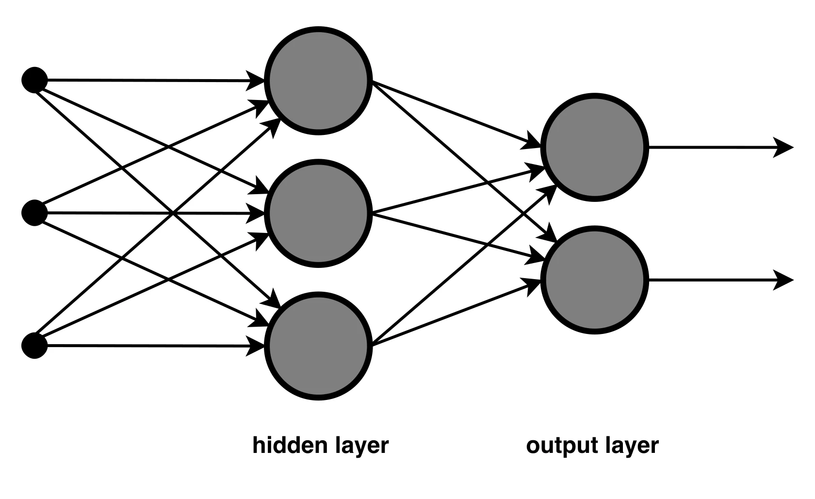
ML includes logistic regression, SVM, random forest, gradient boosting and k‑NN, which usually have relatively few parameters and are simpler to tune. DL refers to architectures such as CNNs, RNNs/LSTMs, Transformers, autoencoders or diffusion networks, where the number of parameters can range from millions to billions. In practice, this translates into a different way of working: in ML, the typical pipeline is data cleaning → feature engineering → model → calibration/interpretation. In DL, you are more likely to encounter elements such as augmentations, GPU training, fine‑tuning and inference optimisation (e.g. batching or TensorRT).

DL is not “always better”, because it can underperform on small datasets or when labels are heavily noisy. In many business tasks on tabular data (e.g. credit scoring), boosting models (XGBoost/LightGBM/CatBoost) often win in terms of accuracy, deployment time and interpretability. ML is also often easier to audit, because you can point to the impact of variables (e.g. SHAP in XGBoost) and decision thresholds. DL is usually harder to explain: tools such as saliency maps or Integrated Gradients can help, but they do not always provide a clear answer to the question “why did the model make that decision?”.

1. 01Feature-based models (ML)Requires feature engineering and a fixed input vector.
2. 02Feature-learning models (DL)Learns representations directly from raw data.
3. 03ML examplesSimpler models (e.g. random forest, regression), fewer parameters.
4. 04DL architecturesComplex networks (e.g. CNNs, Transformers) for image and text.
5. 05Practical approachStart with solid ML, consider DL when there are limitations.

Most importantly: ML relies on defined features, whereas DL learns their representations directly from data, which is crucial for complex data types.

Optymalny wybór metodologii dla różnych typów danych

Choosing the optimal methodology depends first and foremost on the type of data. Tables most often point towards ML, whereas images, text and audio usually require DL. In churn prediction in CRM, ML (e.g. LightGBM) is often the practical choice, because deployment and iteration are faster and simpler. By contrast, in object detection in images, DL (e.g. YOLO) is standard, because networks can learn features directly from pixels. In hybrid solutions (e.g. text description + tabular features), combined approaches work well, such as BERT embeddings + boosting on features or a multimodal network.

• Tabular data: usually ML (LightGBM/CatBoost), because it models non-linearities and interactions well and quickly provides a sensible baseline.
• Unstructured data (images, text, sound): most often DL (CNN/Transformer), because it learns representations from the raw input.
• Little data: more often ML with refined feature engineering and regularisation; in DL, transfer learning is justified (fine‑tuning pre-trained models).
• NLP at small scale: ML with n‑grams and TF‑IDF can work surprisingly well for spam or review classification.

It is worth taking the scale of the data and training costs into account as a decision criterion right from the start. ML often performs well on thousands or tens of thousands of records, and training on CPU usually takes minutes, which makes rapid tests and A/B experiments easier. DL usually “prefers” larger datasets (from tens of thousands in transfer learning to millions when training from scratch) and more often requires GPU/TPU, while individual training runs can take a long time. If time‑to‑value matters, ML usually delivers a useful result faster, while DL is worthwhile when you expect a real quality gain thanks to unstructured data or transfer learning.

The role of features and input data in ML and DL

In ML, the result is most often determined by the quality and design of the features, because the model learns mainly from manually prepared signals. In practice, the question “how do I improve accuracy?” often boils down to “how do I add better variables”, e.g. 7/30-day aggregations, interaction features or target encoding. In DL, quality improvements more often result from better data (more examples, better labels) and augmentation, because the network builds representations from the input on its own. A simple rule of thumb is this: in ML you invest in feature engineering, and in DL in data, labels and augmentations.

Input preparation also differs from a technical perspective, because not all models “like” the same scales and formats. In ML, standardisation is often crucial for SVM, k‑NN and regression (e.g. StandardScaler), while trees and boosting usually do not need it. In DL, the scale of inputs matters, so input normalisation is often used (e.g. mean/std for images) as well as normalisation inside the network (BatchNorm/LayerNorm). Equally important is matching the split to production realities, because an inappropriate validation setup can produce deceptively high metrics.

The way missing values and categorical variables are handled can directly determine which approach is best for tabular data. In ML, missing data is dealt with by imputation (e.g. the median, KNNImputer) or by using more robust models, such as CatBoost, which can treat absence as a signal. In DL, missing values (NaN) are problematic, so they are usually encoded as a separate mask or flag, or methods for tabular data are used (e.g. TabNet) with carefully chosen imputation. For categories in ML, One‑Hot or target encoding are standard, while in DL embeddings are usually used (e.g. 16–128 dimensions), which works well when there are many unique values.

In text and image tasks, the differences in input data are especially clear. In NLP, the ML approach often relies on n-grams and TF-IDF, which can work solidly for spam or review classification at a smaller scale, whereas DL usually uses tokenisation (BPE/WordPiece) and Transformers (e.g. BERT) to better capture context and long-range dependencies. In images, ML quickly loses quality without hand-crafted descriptors (HOG, SIFT) or ready-made features from a pretrained CNN, while DL (CNN/ViT) learns filters directly from pixels. For imbalanced classes, ML often uses class weights, SMOTE or decision threshold adjustment, while DL more often uses focal loss, sample weighting and appropriate batching.

1. 01Feature engineering in MLFeature quality is key. Manual signals, aggregations.
2. 02Data engineering in DLMore data and labels. Augmentation, self-learning.
3. 03Scaling and formatsTechnical adjustment. Standardisation is important in ML.

Rule of thumb: in ML invest in features, in DL — in data and labels.

Comparison of models and architectures: when to choose CNN and when to choose Transformer

CNN is most often chosen for images, and Transformer for text, because their assumptions (inductive bias) suit these types of data well. CNN assumes locality and translational invariance, which makes it easier to learn from pixels and detect patterns regardless of position. Transformer is based on the attention mechanism between tokens, which allows it to model dependencies in sequences accurately. The best choice of architecture is usually the one that “fits” the structure of the data and shortens the model’s path to learning the right dependencies.

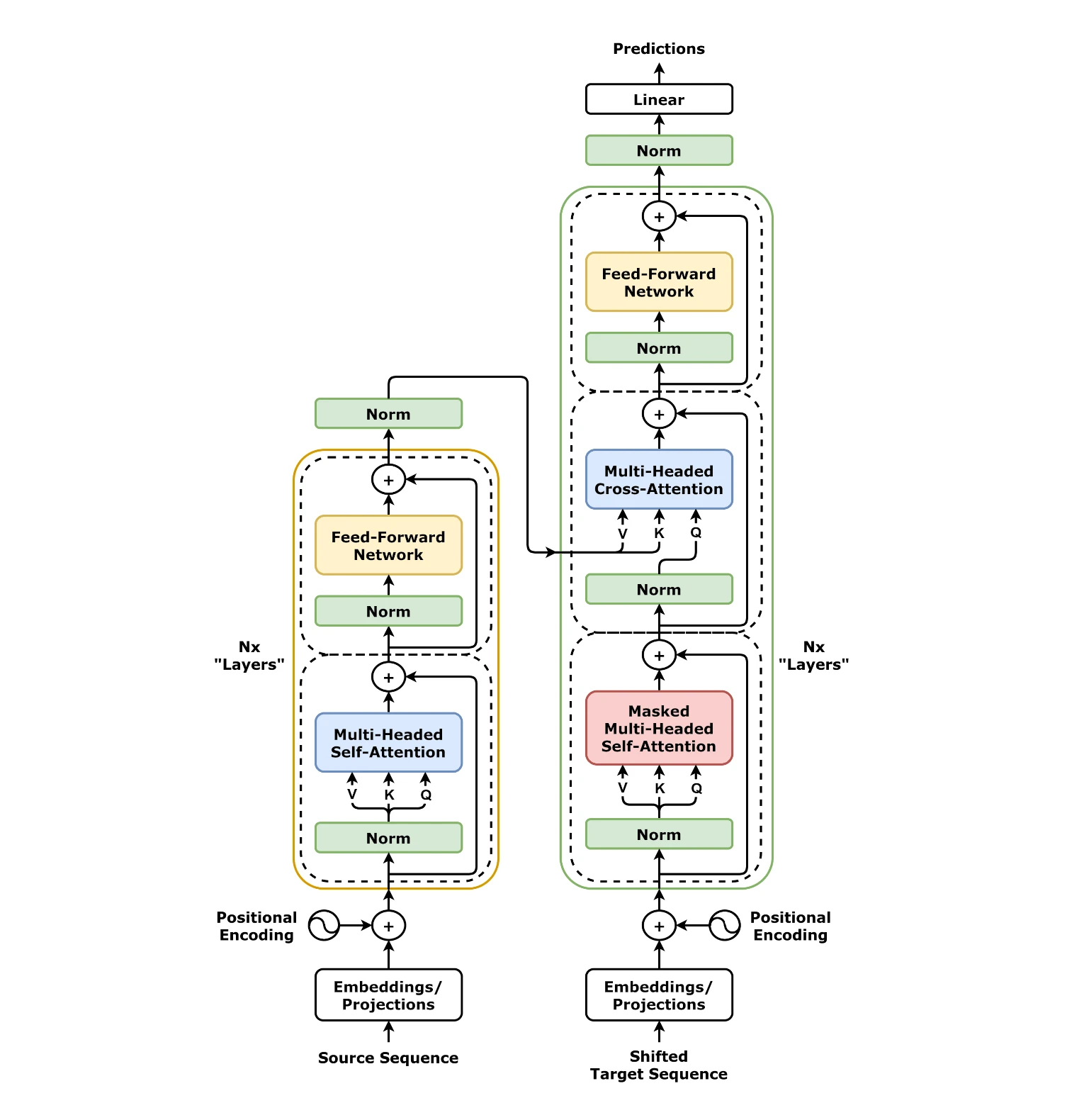
However, Transformer is not “just for text”, because attention can also be calculated between pixels, although this increases the computational cost and deployment requirements. In practice, in DL inputs can have variable sizes (text length, image resolution), so standardisation is needed, such as tokenisation, padding and resizing, as well as latency control. In sequential tasks (e.g. clicks, text), DL makes it possible to model the course of the sequence without manually encoding relationships, but you need to keep an eye on sequence length, masking and the O(n²) cost in attention. This affects both training and inference, especially when response time matters.

The choice between CNN and Transformer is often also tied to the transfer learning strategy, because ready-made representations can significantly shorten the path to production-quality results. In DL, transfer learning can be very effective: you transfer representations from pre-trained models (e.g. ResNet, BERT) and fine-tune them for your own problem. This means you can work sensibly even when you are not training from scratch on millions of examples. At the same time, a change in architecture (e.g. a model variant) affects the number of parameters, memory requirements and training dynamics, so comparisons are best carried out within predefined families of models and checkpoints.

Training and computing resources: how to use GPU effectively

You will make the fullest use of the GPU in deep learning, because it is DL that usually requires acceleration for training and iteration time to make practical sense. In the case of fine-tuning, runtime can range from a dozen minutes to several hours, depending on the batch size and GPU class (e.g. RTX 4090 vs T4), and training from scratch is usually even more expensive. This results from backpropagation, which calculates gradients for millions of parameters and most often requires many epochs. If your goal is rapid iteration, plan experiments so as to shorten the time of a single training run as much as possible and make it easier to compare results.

Effective GPU use in DL most often comes down to choosing training settings in such a way that the batch fits into memory while maintaining stable learning. This is helped by mixed precision training (AMP, FP16/BF16) and techniques such as gradient clipping, an appropriate scheduler (e.g. cosine, linear warmup) and matching the optimiser (e.g. AdamW, SGD). When k-fold is too computationally expensive, a fixed train/val/test split is more often chosen, or runs are repeated with different seeds to assess result stability. In DL, the cost of a validation error is high, so setting the split and controlling the training run (e.g. early stopping) genuinely saves resources.

The GPU is most often “wasted” when it is hard to determine whether an improvement comes from a change in the model or rather from randomness in the data and initialisation. For this reason, in longer training runs experiment monitoring is practically essential and is usually done with tools such as Weights & Biases, MLflow or TensorBoard. If the model “does not work”, DL debugging includes, among other things, checking the loss and gradients, trying to overfit on a small sample, verifying augmentation and tokenisation, and checking numerical stability (e.g. NaN in the loss). These steps make it easier to catch pipeline issues before you start increasing the model size or the number of epochs.

1. 01Deep Learning (DL)Key for acceleration.
2. 02Time and GPU classDepends on hardware and batch.
3. 03BackpropagationMillions of parameters, many epochs.
4. 04Rapid iterationPlan short experiments.
5. 05Memory optimisationAdjust batch, stable learning.

Key: balance training settings to make the most of GPU memory and speed up iterations.

Model interpretability: how to explain business decisions

Business decisions are easiest to justify when you can point to the impact of individual variables and decision thresholds, which usually works to the advantage of classic ML models. In practice, regressions and trees are more readable, and in the case of boosting methods (e.g. XGBoost), SHAP is often used to show the contribution of features to the result. This approach makes it easier to talk to an auditor or client, because the answer to the question “what influenced the decision?” can be linked to specific input variables. If interpretability is a formal requirement, ML usually offers a simpler path to audit than DL.

In DL, explaining decisions is more demanding, because models learn complex representations and it is not always possible to translate them into unambiguous rules. Most often, tools such as saliency maps, Integrated Gradients or LIME are used, and in sequence models attention maps can be helpful. These methods can indicate which parts of the input were important, but their interpretation is often ambiguous and does not always meet formal requirements. In practice, this means that an “explanation” in DL more often supports analysis than provides hard justification for a decision.

Interpretability should be compared with a reliable quality measurement, because both ML and DL have their own evaluation pitfalls. In DL, it is easy to achieve high accuracy with an incorrect data setup (e.g. leakage through augmentations or duplicated images), which makes it harder to defend decisions before stakeholders. In ML, the risk more often concerns incorrect categorical encoding and information leakage through aggregations calculated on the whole dataset rather than on training only. Well-set validation and clear communication of metrics (e.g. AUC, F1, RMSE) help to connect “why did the model decide this way?” with “how do we know it works properly?”.

Choosing an approach: when to go for ML and when for DL

It is safest to reach for ML when you are working with tabular data, have a limited number of examples and need rapid iteration. In such tasks, boosting models (XGBoost/LightGBM/CatBoost) often win in terms of accuracy, deployment time and interpretability, and training can usually be carried out on a CPU in minutes. DL, on the other hand, is more practical when the data is unstructured (images, text, sound) and you want the model to learn representations directly from raw input. If regulatory and audit requirements are critical, ML usually provides a simpler path to showing the influence of variables (e.g. SHAP) and defending decision thresholds.

The choice between ML vs DL is often decided by deployment constraints and maintenance costs, not by quality metrics alone. ML can be deployed efficiently in transactional systems on CPU (e.g. serialisation and microservice architecture), whereas DL more often requires export (ONNX/TorchScript), optimisation (TensorRT/OpenVINO) and keeping latency under control on GPU or on an edge device. In practice, the question “can I afford DL in production?” comes down to calculating the cost per 1000 predictions and the acceptable latency (e.g. 50–200 ms in an application). When the environment is limited to CPU in a legacy system, ML usually turns out to be the safer option.

• Choose ML when you are working with tabular data, time-to-value matters and you want to check the effect quickly (e.g. A/B), and interpretability is also required.
• Choose DL when the data is unstructured or sequential and you need a model that learns features on its own (e.g. CNN/Transformer), especially if you have access to GPU and sufficient data scale.
• Consider transfer learning when you have little data, but can fine-tune a pretrained model (e.g. ResNet, BERT/HerBERT) instead of training from scratch.
• Consider a hybrid approach when you combine different data types (e.g. text + tabular features), such as a BERT embedding + boosting on features or a multimodal network.

The decision is best closed by a pragmatic comparison of “what delivers the greatest return on work” in your context. If the ML result is already “good enough”, and further improvement from DL is marginal (e.g. a slight increase in AUC after a week of experiments), it is often more cost-effective to refine the data, process or decision thresholds than to change the entire model class. In tasks such as credit risk or fraud detection, probability calibration and stability over time are also important, where ML (boosting + calibration) is often simpler to maintain in cyclical re-training. In practice, a sensible strategy is: first a solid ML baseline, and only then DL when the data type or the inability to build good features becomes the limiting factor.

How to handle data limitations and solve quality issues

You can deal with data limitations most easily when you first diagnose the specific problem (too little data, label noise, imbalanced classes, drift), and only then choose the right technique, rather than “adding” model complexity. With a small data scale, ML usually wins thanks to lower capacity and a lower risk of overfitting, while in DL transfer learning (fine-tuning) makes sense, because you are not starting from random weights. If the data is tabular and contains missing values, ML offers simpler solutions (imputation or robust models such as CatBoost), whereas in DL missing values (NaN) often require masks/flags or very careful imputation. It is also crucial to set up validation so that it reflects production, because an incorrect split can produce misleading results.

Label noise is particularly dangerous in DL, because high-capacity networks can “memorise” incorrect annotations during long training. If you suspect that some labels are wrong (e.g. 5–20%), in DL you can use, among other things, cleanlab, robust loss, label smoothing and data review procedures, while at the same time it is worth keeping training under control (e.g. early stopping) and using regularisation. In ML, reducing complexity and validating on certain cases also often helps, so you do not tune the model to the noise itself. When label quality is uncertain, the priority should be to “denoise” the data and validation, because changing the architecture alone rarely solves the problem.

The problem of imbalanced classes requires a different set of tools in ML and DL, but in both approaches you need to carefully watch metrics and thresholds. In ML, class weights (class_weight), SMOTE and decision threshold selection work quickly, whereas in DL people more often reach for focal loss, sample weighting and batching strategies. With an extreme imbalance (e.g. 1:10 000), it is easy to get deceptively good metrics without solid validation data, so the evaluation should be particularly conservative. If it is difficult to improve quality further, sometimes stable calibration and a sensibly set threshold give more than “chasing” accuracy alone.

Drift and out-of-distribution (OOD) data require a process approach, because they cannot be “fixed” with a single trick in the model. DL can be more prone to unexpected behaviour when the domain changes (e.g. new types of images from another device), which is why critical systems use robustness tests, input anomaly detection and domain constraints. In ML, drift is often easier to diagnose thanks to monitoring feature distributions and simple alerts (e.g. PSI, KS test), and the less complex model structure makes rapid re-training and version comparison easier. Ultimately, production quality depends on whether the split and monitoring reflect the real operating conditions of the model, not just a “nice result” offline.